Monitor your Internet Connectivity with Pandas and Python

At somes point you may ask if your Internet Connectivity (for your home, small/medium business, etc.) is working as your provider says it is working. Probably the Internet connection is fine while you are testing it in front of your desktop. But what about two hours later or at night? You do not have the time to test the Internet connection 24/7. So, that is why, it is important to automate the way you monitor your Internet Connectivity.

To accomplish this task, we are going to use PANDAS as the core of the solution together with Pings, Linux shell scripting, Crontab tasks, Python and Jupyter Notebook.

Background

One way to monitor the Internet Connectivity is through PINGs. The whole theory you can find it here. But in summary: An ICMP packet is sent from any local computer to a destination computer on the Internet. And if remote computer responds in less than x [ms], it means the connection is fine at that precise moment.

10 ≤ x ≤ 20 [ms]: If remote computer is close to local network

150 ≤ x ≤ 300 [ms]: If remote computer is in different State, Country or Continent

500 ≤ x ≤ 700 [ms]: Satellite communication

Note. – The values also can vary according to the medium of communication like if it is fiber, DSL, coaxial, etc. But in general, those are good approximately values.

Then. It must be considered the threshold of lost packets. In general, we can consider:

Packet lost < 2%: You have a good Internet Connection

2% <= Packet lost < 5%: A warning signal that something is not quite good with the connection

Packet lost >= 5%: Do something immediately. Your internet connection is really bad.

Practical case of study

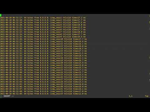
Let’s ping the DNS google server 8.8.8.8

ping -c 100 8.8.8.8

Pings statistics

As you can see the media value is 12.72 [ms]

Let’s group these ICMP request every 5 minutes.

Therefore x[%] of packet lost means:

Considering that a lost packet has a RTT ≥ 2000 [ms]. We can use the following formula to know the equivalent of packet lost into [ms]

Equation deducted by Omar N

So, x[%] of packet lost in [ms] is:

Implementation

Install python3-venv

On Ubuntu

sudo apt-get install python3-venv

On Opensue

zypper install python3-virtualenv

Create the Virtual Environment

mkdir directory-name
cd directory-name
python3 -m venv venv
source venv/bin/activate

Install libraries

pip install pandas
pip install jupyter
pip install matplotlib

Download code from my GitHub

wget https://raw.githubusercontent.com/omarcino/pings-data-analysis/main/pingv4.sh

Make scripting executable

chmod a+x pingv4.sh

Edit pingv4.sh

# Example

host="8.8.8.8"
directory="/root/pings"

Schedule the code to run everytime Linux stars

contrab -e
@reboot /pathdirectory/pingv4.sh

Verify the script is working

tail 2021-05-31.ipv4-8.8.8.8

Start Jupyter Notebook on Linux

jupyter notebook --no-browser --port=8888 --allow-root

You will receive a token value

# Example
http://localhost:8888/?token=dfddfd@#23

Connect Windows Power Shell to Linux Jupyter

ssh -N -f -L localhost:8888:localhost:8888 linux-user00@linux-ip-address

Open Jupyter Notebook on your browser

# Example
http://localhost:8888/?token=tokeyGivenByLinuxServer

Execute Pandas, Python code

### Import libraries ###
%matplotlib inline
import numpy as np
import matplotlib.pyplot as plt
import pandas as pd
import matplotlib.dates as mdates
from matplotlib.dates import DateFormatter
from datetime import date

### Import log ping file ###
# Make sure head is: date time size bytes from ip icmp ttl rtt ms
pings = pd.read_csv("ping-log-file-name", sep=' ', engine='python')

### Formating datetime and rtt time ###
pings['DateTime'] = pings.date + ' ' + pings.time.str.rstrip(":")
pings.DateTime = pings.DateTime.astype('datetime64[ns]')
pings.rtt = pings.rtt.str.strip("time=")
#
# Considering 2000 [ms] as lost packet
pings.rtt = pings.rtt.fillna(2000)
pings.rtt = pings.rtt.astype('float')

### New df that only have DateTime and rtt ###
pings_v2 = pings[['DateTime', 'rtt']].copy()
pings_v2 = pings_v2.set_index(pings_v2.DateTime)

### Getting samples every 5 ### minutes
pings5min = pings_v2.resample('5T').mean()

### To zoom-in unccomment the next line ###
#pings5min = pings5min.loc['2021-05-30 17:00:00':'2021-05-30 19:00:00']

### Re numerate index 0, 1, 2, ... ###
pings5min = pings5min.reset_index(drop=False)

### Create figure and plot ### space
fig, ax = plt.subplots(figsize=(15, 5))

### Add x-axis and y-axis ###
ax.plot(pings5min.DateTime, pings5min.rtt, label='8.8.8.8')
plt.title('Pings - 5/30/21', fontdict={'fontsize': 20})
plt.xlabel('HH:MM')
plt.ylabel('ms')

### Define the date format ###
date_form = DateFormatter('%H:%M')
ax.xaxis.set_major_formatter(date_form)
plt.legend()

### To save graph. Uncomment ### the next line
#plt.savefig('SouthClayton', dpi=300)

### Get the graph ###
plt.show()

Graph examples

Conclusions

• We are able to test our Internet connectivity every single second, 24 hours a day, 7 days a week and so on

• The data collected will be huge. Thousands of thousands of registers

• Applications like Excel are not able to handle that amount of information

• Pandas and Python let us analyze tons of Internet connectivity data in just one sight/two seconds.

• We will have graphs to create reports. And that could be useful, for example, to make claims to our Internet Provider.